install.packages("synapser", repos = c("http://ran.synapse.org"))
install.packages(c("tidyverse", "lubridate"))AD Knowledge Portal Workshop: Download and explore 5XFAD mouse data in RStudio
Overview
We will be working with metadata and RNAseq counts data from The Jax.IU.Pitt_5XFAD Study (Jax.IU.Pitt_5XFAD), which can be found here on the AD Knowledge Portal. During this workshop we will use R to:
Log in to Synapse
Download the counts file (single-file download from Synapse)
Download the metadata files (bulk data download from Synapse)
Map samples in data files to information in metadata files
Explore the data
Setup
Install and load packages
If you haven’t already, install synapser (the Synapse R client), as well as the tidyverse family of packages. The “tidyverse” package is shorthand for installing a bunch of packages we need for this notebook (dplyr, ggplot2, purrr, readr, stringr, tibble). It also installs “forcats” and “tidyr”, which are not used in this notebook.
Load libraries
library(synapser)
library(dplyr)
library(purrr)
library(readr)
library(lubridate)
library(stringr)
library(tibble)
library(ggplot2)Login to Synapse
Next, you will need to log in to your Synapse account.
Login option 1: Synapser takes credentials from your Synapse web session
If you are logged into the Synapse web browser, synapser will automatically use your login credentials to log you in during your R session! All you have to do is call synLogin() from a script or the R console.
synLogin()Login option 2: Synapse PAT
Follow these instructions to generate a Personal Access Token, then paste the PAT into the code below. Make sure you scope your access token to allow you to View, Download, and Modify.
⚠ DO NOT put your Synapse access token in scripts that will be shared with others, or they will be able to log in as you.
synLogin(authToken = "<paste your personal access token here>")For more information on managing Synapse credentials with synapser, see the documentation here.
Download data
While you can always download data from the AD Portal website via your web browser, it’s usually faster and often more convenient to download data programmatically.
Download a single file
To download a single file from the AD Knowledge Portal, you can click the linked file name to go to a page in the Synapse platform where that file is stored. Using the synID on that page, you can call the synGet() function from synapser to download the file.
Exercise 1: Use Explore Data to find processed RNAseq data from the Jax.IU.Pitt_5XFAD Study
This filters the table to a single file. In the “Id” column for this htseqcounts_5XFAD.txt file, there is a unique Synapse ID (synID).

We can then use that synID to download the file. Some information about the file and its storage location within Synapse is printed to the R console when we call synGet.
counts_id <- "syn22108847"
synGet(counts_id,
downloadLocation = "files/",
ifcollision = "overwrite.local") # Prevents making multiple copiesThe argument ifcollision = "overwrite.local" means that instead of downloading the file and saving it as a new copy, it will overwrite the current file at that location if it already exists, to avoid cluttering your hard drive with multiple copies of the same file. Before downloading, synGet will check if the file on your hard drive is the same as the version on Synapse, and will only download from Synapse if the two files are different.
This is very useful for large files especially: you can ensure that you always have the latest copy of a file from Synapse, without having to re-download the file if you already have the current version on your hard drive.
Let’s take a quick look at the file we just downloaded. Calling a tibble object will print the first ten rows in a nice tidy output; doing the same for a base R dataframe will print the whole thing until it runs out of memory. If you want to inspect a large dataframe, use head(df).
counts <- read_tsv("files/htseqcounts_5XFAD.txt", show_col_types = FALSE)
head(counts)Bulk download files
Exercise 2: Use Explore Studies to find all metadata files from the Jax.IU.Pitt_5XFAD study
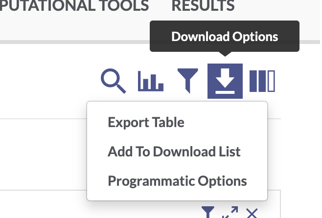
Use the facets and search bar to look for data you want to download from the AD Knowledge Portal. Once you’ve identified the files you want, click on the download arrow icon on the top right of the Explore Data table and select “Programmatic Options” from the drop-down menu.
In the window that pops up, select the “R” tab from the top menu bar. This will display some R code that constructs a SQL query of the Synapse data table that drives the AD Knowledge Portal. This query will allow us to download only the files that meet our search criteria.
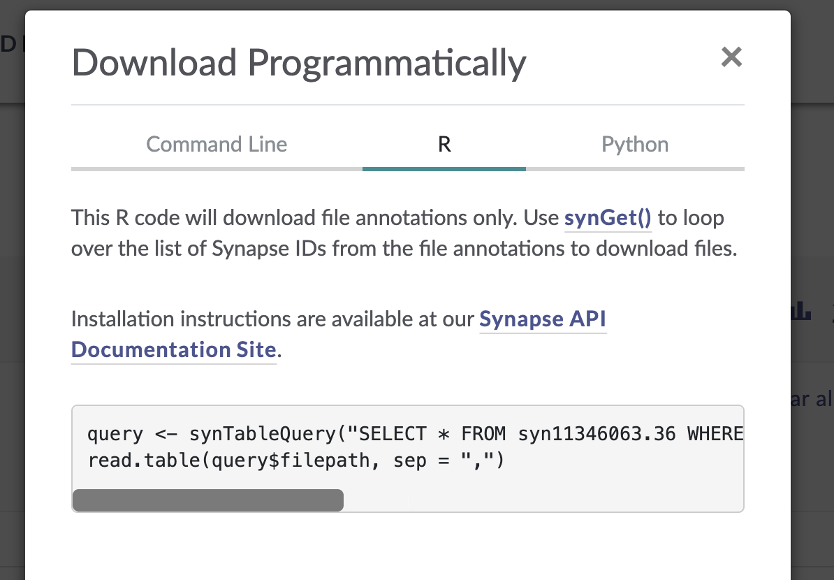
We’ll download our files using two steps:
We will use the
synTableQuery()code the portal gave us to download a CSV file that lists all of the files we want. This CSV file is a table, one row per file in the list, containing the Synapse ID, file name, annotations, etc associated with each file.- This does NOT download the files themselves. It only fetches a list of the files plus their annotations for you.
We will call
synGet()on each Synapse ID in the table to download the files.
Why isn’t this just one step instead of two?
Splitting this into steps can be extremely helpful for cases where you might not want to download all of the files back-to-back. For example, if the file sizes are very large or if you are downloading hundreds of files. Downloading the table first lets you: a) Fetch helpful annotations about the files without downloading them first, and b) do things like loop through the list one by one, download a file, do some processing, and delete the file before downloading the next one to save hard drive space.
Back to downloading…
The function synTableQuery() returns a Synapse object wrapper around the CSV file, which is automatically downloaded to a folder called .synapseCache in your home directory. You can use query$filepath to see the path to the file in the Synapse cache.
# download the results of the filtered table query
query_string <- paste(
"SELECT * FROM syn11346063 WHERE (( `study` HAS ( 'Jax.IU.Pitt_5XFAD' ))",
"AND ( `resourceType` = 'metadata' ) )"
)
query <- synTableQuery(query_string, includeRowIdAndRowVersion = FALSE)Downloaded syn11346063 to /Users/jbeck/.synapseCache/749/149695749/SYNAPSE_TABLE_QUERY_149695749.csv# view the file path of the resulting csv
query$filepath[1] "/Users/jbeck/.synapseCache/749/149695749/SYNAPSE_TABLE_QUERY_149695749.csv"We’ll use read_csv (from the readr package) to read the CSV file into R (although the provided read.table or any other base R version is also fine!). We can explore the download_table object and see that it contains information on all of the AD Portal data files we want to download. Some columns like the “id” and “parentId” columns contain info about where the file is in Synapse, and some columns contain AD Portal annotations for each file, like “dataType”, “specimenID”, and “assay”. This annotation table will later allow us to link downloaded files to additional metadata variables!
# read in the table query csv file
download_table <- read_csv(query$filepath, show_col_types = FALSE)
download_tableLet’s look at a subset of columns that might be useful:
download_table %>%
dplyr::select(id, name, metadataType, assay, fileFormat, currentVersion)Tip: Copy this file and save it somewhere memorable to have a complete record of all the files you are using and what version of each file was downloaded – for reproducibility!
Finally, we use a mapping function from the purrr package to loop through the “id” column and apply the synGet() function to each file’s synID. In this case, we use purrr::walk() because it lets us call synGet() for its side effect (downloading files to a location we specify), and returns nothing.
# loop through the column of synIDs and download each file
purrr::walk(download_table$id, ~synGet(.x, downloadLocation = "files/",
ifcollision = "overwrite.local"))You can also do this as a for loop, i.e.:
for (syn_id in download_table$id) {
synGet(syn_id,
downloadLocation = "files/",
ifcollision = "overwrite.local")
}Congratulations, you have bulk downloaded files from the AD Knowledge Portal!
✏ Note on download speeds
For situations where you are downloading many large files, the R client performs substantially slower than the command line client or the Python client. In these cases, you can use the instructions and code snippets for the command line or Python client provided in the “Programmatic Options” menu.
✏ Note on file versions
All files in the AD Portal are versioned, meaning that if the file represented by a particular synID changes, a new version will be created. You can access a specific versions by using the version argument in synGet(). More info on version control in the AD Portal and the Synapse platform can be found here.
Single-specimen files
For files that contain data from a single specimen (e.g. raw sequencing files, raw mass spectra, etc.), we can use the Synapse annotations to associate these files with the appropriate metadata.
Excercise 3: Use Explore Data to find all RNAseq files from the Jax.IU.Pitt_5XFAD study.
If we filter for data where Study = “Jax.IU.Pitt_5XFAD” and Assay = “rnaSeq” we will get a list of 148 files, including raw fastqs and processed counts data.
Synapse entity annotations
We can use the function synGetAnnotations to view the annotations associated with any file before actually downloading the file.
# the synID of a random fastq file from this list
random_fastq <- "syn22108503"
# extract the annotations as a nested list
fastq_annotations <- synGetAnnotations(random_fastq)
head(fastq_annotations)$sex
[1] "female"
$room
[1] "JAX_MGL373"
$assay
[1] "rnaSeq"
$grant
[1] "U54AG054345"
$organ
[1] "brain"
$study
[1] "Jax.IU.Pitt_5XFAD"The file annotations let us see which study the file is associated with (Jax.IU.Pitt.5XFAD), which species it’s from (Mouse), which assay generated the file (rnaSeq), and a whole bunch of other properties. Most importantly, single-specimen files are annotated with with the specimenID of the specimen in the file, and the individualID of the individual that specimen was taken from. We can use these annotations to link files to the rest of the metadata, including metadata that is not in annotations. This is especially helpful for human studies, as potentially identifying information like age, race, and diagnosis is not included in file annotations.
ind_meta <- read_csv("files/Jax.IU.Pitt_5XFAD_individual_metadata.csv",
show_col_types = FALSE)
# find records belonging to the individual this file maps to in our joined metadata
filter(ind_meta, individualID == fastq_annotations$individualID[[1]])Annotations during bulk download
When bulk downloading many files, the best practice is to preserve the download manifest that is generated which lists all the files, their synIDs, and all their annotations. If using the Synapse R client, follow the instructions in the Bulk download files section above.
If we use the “Programmatic Options” tab in the AD Portal download menu to download all 148 rnaSeq files from the 5XFAD study, we would get a table query that looks like this:
query_str <- paste(
"SELECT * FROM syn11346063 WHERE ( ( \"study\" HAS ( 'Jax.IU.Pitt_5XFAD' ) )",
"AND ( \"assay\" HAS ( 'rnaSeq' ) ) )"
)
query <- synTableQuery(query_str, includeRowIdAndRowVersion = FALSE)Downloaded syn11346063 to /Users/jbeck/.synapseCache/754/149695754/SYNAPSE_TABLE_QUERY_149695754.csvAs we saw previously, this downloads a csv file with the results of our AD Portal query. Opening that file lets us see which specimens are associated with which files:
annotations_table <- read_csv(query$filepath, show_col_types = FALSE)
annotations_tableYou could then use purrr::walk(download_table$id, ~synGet(.x, downloadLocation = <your-download-directory>)) to walk through the column of synIDs and download all 148 files. However, because these are large files, it might be preferable to use the Python client or command line client for increased speed.
Multispecimen files
Multispecimen files in the AD Knowledge Portal are files that contain data or information from more than one specimen. They are not annotated with individualIDs or specimenIDs, since these files may contain numbers of specimens that exceed the annotation limits. These files are usually processed or summary data (gene counts, peptide quantifications, etc), and are always annotated with isMultiSpecimen = TRUE.
If we look at the processed data files in the table of 5XFAD RNAseq file annotations we just downloaded, we will see that isMultiSpecimen = TRUE, but individualID and specimenID are blank:
annotations_table |>
filter(fileFormat == "txt") |>
dplyr::select(name, individualID, specimenID, isMultiSpecimen)Note: |> is the base R pipe operator. If you are unfamiliar with the pipe, think of it as a shorthand for “take this (the preceding object) and do that (the subsequent command)”. See here for more info on piping in R.
The multispecimen file should contain a row or column of specimenIDs that correspond to the specimenIDs used in a study’s metadata, as we have seen with the 5XFAD counts file.
colnames(counts)[1:20] [1] "gene_id" "32043rh" "32044rh" "32046rh" "32047rh" "32048rh" "32049rh"
[8] "32050rh" "32052rh" "32053rh" "32057rh" "32059rh" "32061rh" "32062rh"
[15] "32065rh" "32067rh" "32068rh" "32070rh" "32073rh" "32074rh"Working with AD Portal metadata
Metadata basics
We have now downloaded several metadata files and an RNAseq counts file from the portal. For our next exercises, we want to read those files in as R data so we can work with them.
We can see from the download_table we got during the bulk download step that we have five metadata files. Two of these should be the individual and biospecimen files, and three of them are assay metadata files.
download_table |>
dplyr::select(name, metadataType, assay)We are only interested in RNAseq data, so we will only read in the individual, biospecimen, and RNAseq assay metadata files.
Now we can read all the metadata files in to R as data frames.
# individual metadata
ind_meta <- read_csv("files/Jax.IU.Pitt_5XFAD_individual_metadata.csv",
show_col_types = FALSE)
# biospecimen metadata
bio_meta <- read_csv("files/Jax.IU.Pitt_5XFAD_biospecimen_metadata.csv",
show_col_types = FALSE)
# assay metadata
rna_meta <- read_csv("files/Jax.IU.Pitt_5XFAD_assay_RNAseq_metadata.csv",
show_col_types = FALSE)✏ Note on best practices
We’ve been using the ifcollision = "overwrite.local" argument to synGet() to avoid making multiple copies of each file, so hard-coding the file names in the code block above works as expected. However, if you forget this argument or the file gets renamed on Synapse, you could be reading in an old file instead of the one you just downloaded!
synGet() returns an object that contains the file path of the downloaded file, and it’s good practice to use this instead to avoid accidentally reading the wrong file. Some code to do this with the metadata files is below (but not executed in this notebook).
# "sapply" loops through each item, applies the function to each one, and returns
# a vector of results.
file_paths <- sapply(download_table$id, function(syn_id) {
syn_obj <- synGet(syn_id,
downloadLocation = "files/",
ifcollision = "overwrite.local")
return(syn_obj$path)
})
# See which files we want
print(file_paths)
ind_meta <- read_csv(file_paths[3], show_col_types = FALSE)
bio_meta <- read_csv(file_paths[4], show_col_types = FALSE)
rna_meta <- read_csv(file_paths[5], show_col_types = FALSE)Verify file contents
At this point we have downloaded and read in the counts file and 3 metadata files into the variables counts, ind_meta, bio_meta, and rna_meta.
Let’s examine the data and metadata files a bit before we begin our analyses.
Counts data
head(counts)The counts data file has a column of Ensembl gene ids and then a bunch of columns with count data, where the column headers correspond to the specimenIDs. These specimenIDs should all be in the RNAseq assay metadata file, so let’s check.
head(rna_meta)Are all the column headers from the counts matrix (except the first “gene_id” column) in the assay metadata?
all(colnames(counts[-1]) %in% rna_meta$specimenID)[1] TRUEAssay metadata
The assay metadata contains information about how data was generated on each sample in the assay. Each specimenID represents a unique sample. We can use some tools from dplyr to explore the metadata.
How many unique specimens were sequenced?
n_distinct(rna_meta$specimenID)[1] 72Were the samples all sequenced on the same platform?
distinct(rna_meta, platform)Biospecimen metadata
The biospecimen metadata contains specimen-level information, including organ and tissue the specimen was taken from, how it was prepared, etc. Each specimenID is mapped to an individualID.
head(bio_meta)All specimens from the RNAseq assay metadata file should be in the biospecimen file…
all(rna_meta$specimenID %in% bio_meta$specimenID)[1] TRUE…But the biospecimen file also contains specimens from different assays.
all(bio_meta$specimenID %in% rna_meta$specimenID)[1] FALSEIndividual metadata
The individual metadata contains information about all the individuals in the study, represented by unique individualIDs. For humans, this includes information on age, sex, race, diagnosis, etc. For MODEL-AD mouse models, the individual metadata has information on model genotypes, stock numbers, diet, and more.
head(ind_meta)All individualIDs in the biospecimen file should be in the individual file
all(bio_meta$individualID %in% ind_meta$individualID)[1] TRUEWhich model genotypes are in this study?
distinct(ind_meta, genotype)Joining metadata
We use the three-file structure for our metadata because it allows us to store metadata for each study in a tidy format. Every line in the assay and biospecimen files represents a unique specimen, and every line in the individual file represents a unique individual. This means the files can be easily joined by specimenID and individualID to get all levels of metadata that apply to a particular data file. We will use the left_join() function from the dplyr package, and the base R pipe operator |>.
# join all the rows in the assay metadata that have a match in the biospecimen metadata
joined_meta <- rna_meta |> #start with the rnaseq assay metadata
#join rows from biospecimen that match specimenID
left_join(bio_meta, by = "specimenID") |>
# join rows from individual that match individualID
left_join(ind_meta, by = "individualID")
joined_metaWe now have a very wide dataframe that contains all the available metadata on each specimen in the RNAseq data from this study. This procedure can be used to join the three types of metadata files for every study in the AD Knowledge Portal, allowing you to filter individuals and specimens as needed based on your analysis criteria!
RNASeq data exploration
We will use the counts data and metadata to do some basic exploratory analysis of gene expression in the Jax 5XFAD mouse model.
Explore covariates
Which covariates from the metadata are we interested in?
# all samples are from the same organ and tissue, so we can probably discard those
distinct(joined_meta, organ, tissue, sampleStatus)# we have different sexes and genotypes, so we are probably interested in those
distinct(joined_meta, sex, genotype)For this example, we will plot gene expression by sex, genotype, and age.
Create timepoint column
The MODEL-AD individual mouse metadata contains columns with birth date and death date for each mouse. Using the RNASeq methods description from the Jax 5XFAD study page in the AD Portal, we expect this data to have equal numbers of individuals sampled at 4, 6, and 12 month timepoints. We can create a new column that captures this info in our joined metadata.
Note: MODEL-AD studies added to the portal after June 2021 include an ‘ageDeath’ column that makes this simpler.
# Convert columns of strings to month-date-year format using the lubridate package
joined_meta_time <- joined_meta |>
mutate(dateBirth = mdy(dateBirth),
dateDeath = mdy(dateDeath)) |>
# create a new column that subtracts dateBirth from dateDeath in days, then
# divide by 30 to get months
mutate(timepoint = as.numeric(difftime(dateDeath, dateBirth,
units = "days")) / 30) |>
# convert numeric ages to timepoint categories
mutate(timepoint = case_when(timepoint > 10 ~ "12 mo",
timepoint < 10 & timepoint > 5 ~ "6 mo",
timepoint < 5 ~ "4 mo"))We now have balanced samples across sex, genotype, and age:
# check that the timepoint column looks ok
joined_meta_time |>
group_by(sex, genotype, timepoint) |>
dplyr::count()Subset covariates
To reduce the width of the dataframe, we will subset only the columns that contain covariates we’re interested in exploring further. Retaining the individualID and specimenID columns will make sure we can map the covariates to the data and back to the original metadata if needed!
# many packages have a "select" function that masks dplyr so we have to specify
covars <- joined_meta_time |>
dplyr::select(individualID, specimenID, sex, genotype, timepoint)
# check the result
covarsConvert ensembleIDs to common gene names
Return to the gene counts matrix we read in earlier. 5XFAD mice express human APP and PSEN1, and the counts matrix includes these human genes (recognizable as starting with ENSG instead of ENSMUS):
counts |>
filter(!str_detect(gene_id, "MUS"))We will have to manually add gene symbols for the human genes, but we can automatically get the Ensembl ID to gene symbol mapping for all of the mouse genes. There are many possible ways to do this in R. Below are two options:
1. BiomaRt option:
OPTIONAL: Transform the Ensembl IDs in the matrix to common gene names, using the R package biomaRt (note: must specify to use the mouse database, although the two genes in the 5XFAD model we identified above are humanized and won’t be translated by the program).
For this option, use the BioconductoR package manager to install biomaRt.
if (!requireNamespace("BiocManager", quietly = TRUE))
install.packages("BiocManager")
BiocManager::install("biomaRt")
library(biomaRt)⚠️ The next two code chunks will not automatically execute in this notebook because they can take a long time – the code is included if you’d like to try this on your own.
We will use the two custom functions below to convert ensemblIDs to gene names:
# This function uses biomaRt and converts ensemblIDs to HGNC names
convertEnsemblToHgnc <- function(ensemblIds) {
ensembl <- biomaRt::useMart('ENSEMBL_MART_ENSEMBL',
dataset = 'mmusculus_gene_ensembl')
genes <- getBM(attributes = c('ensembl_gene_id', 'external_gene_name'),
filters = 'ensembl_gene_id',
values = ensemblIds,
mart = ensembl)
return(genes)
}
# This function calls the previous function and further converts HGNC names to
# Gene symbols
Make.Gene.Symb <- function(GeneENSG) {
GeneConv <- convertEnsemblToHgnc(GeneENSG)
rownames(GeneConv) <- GeneConv$ensembl_gene_id
# If the Ensembl ID wasn't found in the BioMart query, the symbol will be NA
# for that ID. Otherwise this will match symbols to gene names and return them
# in the same order as GeneENSG.
Symb <- GeneConv[GeneENSG, "external_gene_name"]
return(Symb)
}Call the Make.Gene.Symb() function to add a new column with short gene names to our counts dataframe. This will take a minute – there are over 55k genes in our matrix!
named_counts <- counts |>
# The ".after" argument puts the new gene_name column right after the gene_id column
mutate(gene_name = Make.Gene.Symb(gene_id), .after = gene_id)
head(named_counts)2. Pre-translated option:
For this demonstration, instead of running biomaRt, which can be unreliable at times and take a long time to respond, we will append a dataframe to our counts matrix with short gene names already translated
ensembl_to_gene <- read.csv(file = "ensembl_translation_key.csv")
named_counts <- counts %>%
dplyr::left_join(ensembl_to_gene, by = "gene_id") %>%
relocate(gene_name, .after = gene_id)
head(named_counts)How many genes are missing a gene symbol?
sum(is.na(named_counts$gene_name) | nchar(named_counts$gene_name) == 0)[1] 3907Are all the gene names unique?
non_na_genes <- named_counts$gene_name[!is.na(named_counts$gene_name) &
nchar(named_counts$gene_name) > 0]
length(non_na_genes) - n_distinct(non_na_genes)[1] 55We need to clean up the humanized gene names and append unique identifiers to the duplicate names.
# The first two genes in the matrix are the humanized genes PSEN1 (ENSG00000080815)
# and APP (ENSG00000142192). Set these manually:
named_counts[1, "gene_name"] <- "PSEN1"
named_counts[2, "gene_name"] <- "APP"
# Make all gene names unique and remove unneeded column
named_counts <- named_counts |>
# Replace NA symbols, make all symbols unique
mutate(gene_name = replace(gene_name, is.na(gene_name), "UNKNOWN"),
gene_name = replace(gene_name, gene_name == "", "UNKNOWN"),
gene_name = make.unique(gene_name)) |>
# Throw away Ensembl IDs
dplyr::select(-gene_id) |>
# Set rownames to gene_name, also removes the gene_name column
column_to_rownames(var = "gene_name")
head(named_counts)Transpose counts matrix and join to covariates
Now we can transpose the dataframe so that each row contains count data cross all genes for an individual, and join our covariates by specimenID.
counts_tposed <- named_counts |>
t() |> # transposing also forces the df to a matrix
as_tibble(rownames = "specimenID") |> # reconvert to tibble and specify rownames
left_join(covars, by = "specimenID") # join covariates by specimenID# check the transposed matrix looks ok
head(counts_tposed)Let’s check that the covariates got included at the end by cutting out most of the genes:
counts_tposed %>%
dplyr::select(1:3, which(colnames(.) %in% colnames(covars))) %>%
head()Visualize gene count data
Create simple box plots showing counts by genotype and time point, faceted by sex.
# first make the timepoints column a factor and re-order the levels
counts_tposed$timepoint <- factor(counts_tposed$timepoint,
levels = c("4 mo", "6 mo", "12 mo"))Use ggplot to plot gene counts for each specimen by age, sex, and genotype.
# Look at APP levels -- this model is the 5X FAD mutant, so we expect it to be high!
g <- counts_tposed |>
ggplot(aes(x = timepoint, y = APP, color = genotype)) +
geom_boxplot() +
geom_point(position = position_jitterdodge()) +
facet_wrap( ~ sex) +
theme_bw() +
scale_color_manual(values = c("tomato3", "dodgerblue3"))
g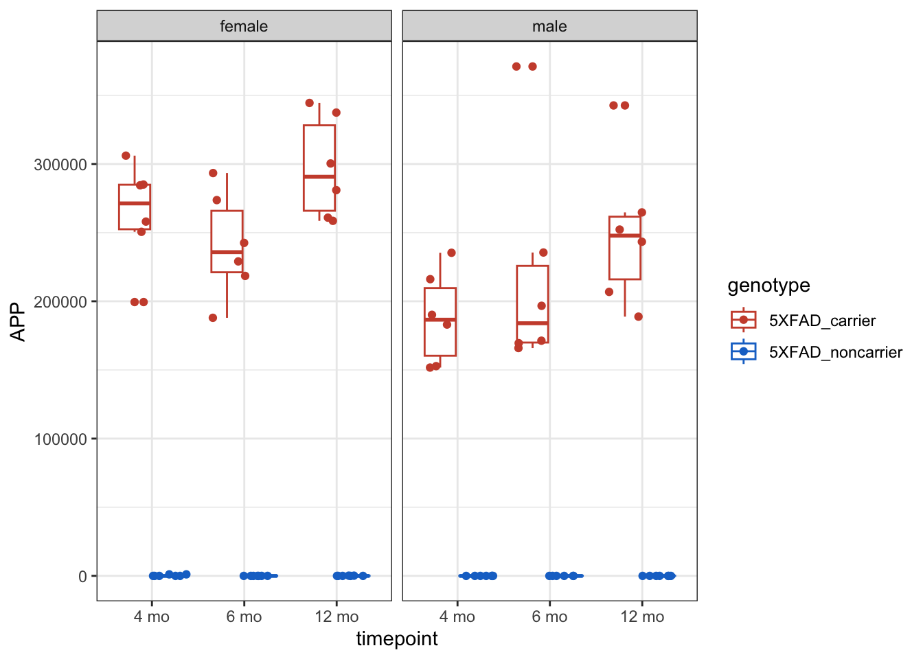
Examine any gene of interest by setting the y argument in the ggplot(aes() mapping equal to the gene name. Ex: y = Trem2
g <- counts_tposed |>
ggplot(aes(x = timepoint, y = Trem2, color = genotype)) +
geom_boxplot() +
geom_point(position = position_jitterdodge()) +
facet_wrap( ~ sex) +
theme_bw() +
scale_color_manual(values = c("tomato3", "dodgerblue3"))
g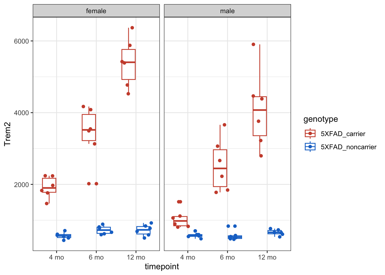
Ex: y = Apoe
g <- counts_tposed |>
ggplot(aes(x = timepoint, y = Apoe, color = genotype)) +
geom_boxplot() +
geom_point(position = position_jitterdodge()) +
facet_wrap( ~ sex) +
theme_bw() +
scale_color_manual(values = c("tomato3", "dodgerblue3"))
g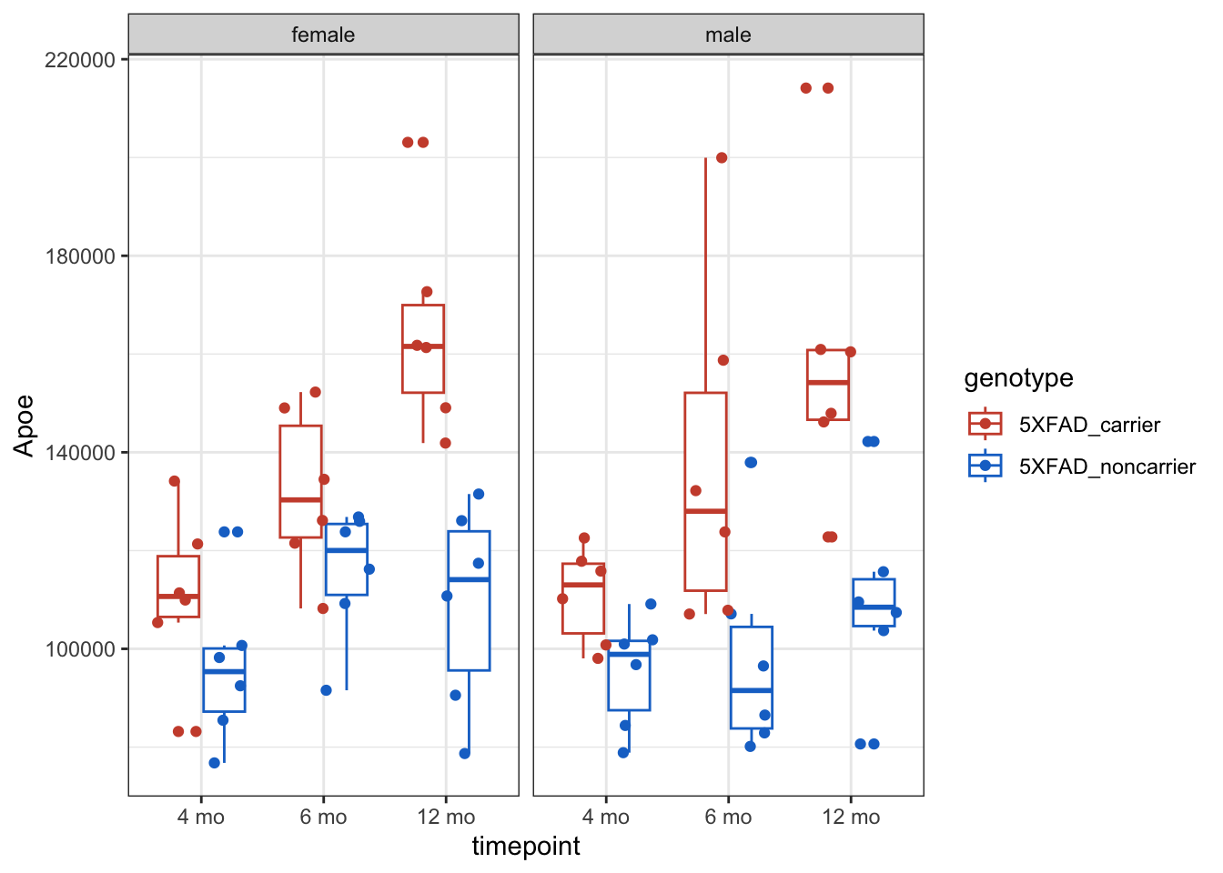

R Package Info
sessionInfo()R version 4.4.1 (2024-06-14)
Platform: aarch64-apple-darwin20
Running under: macOS Monterey 12.7.6
Matrix products: default
BLAS: /Library/Frameworks/R.framework/Versions/4.4-arm64/Resources/lib/libRblas.0.dylib
LAPACK: /Library/Frameworks/R.framework/Versions/4.4-arm64/Resources/lib/libRlapack.dylib; LAPACK version 3.12.0
locale:
[1] en_US.UTF-8/en_US.UTF-8/en_US.UTF-8/C/en_US.UTF-8/en_US.UTF-8
time zone: America/Los_Angeles
tzcode source: internal
attached base packages:
[1] stats graphics grDevices utils datasets methods base
other attached packages:
[1] ggplot2_3.5.1 tibble_3.2.1 stringr_1.5.1 lubridate_1.9.3
[5] readr_2.1.5 purrr_1.0.2 dplyr_1.1.4 synapser_2.1.1.259
loaded via a namespace (and not attached):
[1] utf8_1.2.4 generics_0.1.3 stringi_1.8.4 lattice_0.22-6
[5] hms_1.1.3 digest_0.6.37 magrittr_2.0.3 evaluate_1.0.1
[9] grid_4.4.1 timechange_0.3.0 fastmap_1.2.0 rprojroot_2.0.4
[13] jsonlite_1.8.9 Matrix_1.7-0 fansi_1.0.6 scales_1.3.0
[17] codetools_0.2-20 cli_3.6.3 crayon_1.5.3 rlang_1.1.4
[21] bit64_4.5.2 munsell_0.5.1 withr_3.0.1 yaml_2.3.10
[25] parallel_4.4.1 tools_4.4.1 tzdb_0.4.0 colorspace_2.1-1
[29] here_1.0.1 reticulate_1.39.0 vctrs_0.6.5 R6_2.5.1
[33] png_0.1-8 lifecycle_1.0.4 htmlwidgets_1.6.4 bit_4.5.0
[37] vroom_1.6.5 pkgconfig_2.0.3 pillar_1.9.0 gtable_0.3.5
[41] glue_1.8.0 Rcpp_1.0.13 xfun_0.48 tidyselect_1.2.1
[45] rstudioapi_0.16.0 knitr_1.48 farver_2.1.2 rjson_0.2.21
[49] htmltools_0.5.8.1 labeling_0.4.3 rmarkdown_2.28 compiler_4.4.1